Ordinary differential equations (ODE) code
Euler method
We will mainly use ordinary differential equations of the form.
Here \(\vec{x}\) is a vector of state variables at time \(t\). The parameters of the system are represented by the vector \(\vec{p}\).
In one dimension, the system is written as
And the time-invariant steady states are
The stability of the steady state is determined by the derivative:
The simplest way to solve the equation numerically is the Euler integration
We obtain
Starting from an initial value \(x_0\) at time \(t=0\) the solution can now be determined for later time points.
It is of importance to consider the error of the method. The Euler method introduces an error of \({\cal O}(\Delta t^2)\) per integration step. To obtain the solution \(x(t)\) at a time \(t=T\), \(N=T/\Delta t\) integration steps have to be performed. The total error is therefore of the order \({\cal O}(T \Delta t)\) and decreases with decreasing \(\Delta t\). Euler integration is a first-order method. The method is rarely used in real life (too inefficient).
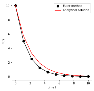
Example Euler Method
We now solve a simple example system with the Euler Method
For \(k>0\) the equation has a stable fix-point at \(x=0\).
The analytical solution at time \(t\) is
We now write a simple function that compares the numerical integration of the simple system with the (known) analytical solution.
%matplotlib inline
import numpy as np
from matplotlib import pyplot as plt

def EulerIntegrator(f_dydt, y0, t_span, N):
    """ The function integrates the simple
    system dx/dt = -k x to a time T using the
    Euler method (N Steps) and initial condition x0.

    param f_dydt: ode system as f(y,t) which returns dy/dt
    param y0: initial values
    param t_span: 2-tuple of floats, interval of integration
    param N: number of time points

    usage: x = SimpleEuler(f, y0, [t_start, t_end], N)
    """
    k = 1 # set parameter k

    # some parameters
    T = float(t_span[1] - t_span[0])
    dt = T/N
    time_vec = np.linspace(t_span[0], t_span[1], num=N)
    x = [float(y0)]

    # integration
    y_vec = []
    for k, t in enumerate(time_vec):
        if k == 0:
            y = y0
        else:
            y = y + dt * f_dydt(y,t)
        y_vec.append(y)

    return y_vec, time_vec


def exponential_decay(y, t):
    """ Linear 1 dimensional ODE"""
    dydt = -0.5 * y
    return dydt

y0 = 10.0

y, t = EulerIntegrator(exponential_decay, y0=y0, t_span=[0,10], N=10)

# plot Euler and exact solution
fig, ax = plt.subplots(nrows=1, ncols=1, figsize=(5,5))

ax.plot(t, y, 'ko-', markersize=8, label='Euler method')
ax.plot(t, y0*np.exp(-0.5*t),'r-',label='analytical solution')

ax.set_xlabel('time t')
ax.set_ylabel('x(t)')
ax.legend(loc='upper right')
plt.show()
Numerical integration in python
The module scipy.integrate offers a variety of build-in functions
for numerical integration. We will mainly solve_ivp (formerly
odeint) for numerical integration.
See also: https://docs.scipy.org/doc/scipy/reference/generated/scipy.integrate.solve_ivp.html
from scipy.integrate import solve_ivp
help(solve_ivp)
Help on function solve_ivp in module scipy.integrate._ivp.ivp: solve_ivp(fun, t_span, y0, method='RK45', t_eval=None, dense_output=False, events=None, vectorized=False, args=None, **options) Solve an initial value problem for a system of ODEs. This function numerically integrates a system of ordinary differential equations given an initial value:: dy / dt = f(t, y) y(t0) = y0 Here t is a one-dimensional independent variable (time), y(t) is an n-dimensional vector-valued function (state), and an n-dimensional vector-valued function f(t, y) determines the differential equations. The goal is to find y(t) approximately satisfying the differential equations, given an initial value y(t0)=y0. Some of the solvers support integration in the complex domain, but note that for stiff ODE solvers, the right-hand side must be complex-differentiable (satisfy Cauchy-Riemann equations [11]_). To solve a problem in the complex domain, pass y0 with a complex data type. Another option always available is to rewrite your problem for real and imaginary parts separately. Parameters ---------- fun : callable Right-hand side of the system. The calling signature isfun(t, y). Here t is a scalar, and there are two options for the ndarray y: It can either have shape (n,); then fun must return array_like with shape (n,). Alternatively it can have shape (n, k); then fun must return an array_like with shape (n, k), i.e. each column corresponds to a single column in y. The choice between the two options is determined by vectorized argument (see below). The vectorized implementation allows a faster approximation of the Jacobian by finite differences (required for stiff solvers). t_span : 2-tuple of floats Interval of integration (t0, tf). The solver starts with t=t0 and integrates until it reaches t=tf. y0 : array_like, shape (n,) Initial state. For problems in the complex domain, pass y0 with a complex data type (even if the initial value is purely real). method : string or OdeSolver, optional Integration method to use: * 'RK45' (default): Explicit Runge-Kutta method of order 5(4) [1]_. The error is controlled assuming accuracy of the fourth-order method, but steps are taken using the fifth-order accurate formula (local extrapolation is done). A quartic interpolation polynomial is used for the dense output [2]_. Can be applied in the complex domain. * 'RK23': Explicit Runge-Kutta method of order 3(2) [3]_. The error is controlled assuming accuracy of the second-order method, but steps are taken using the third-order accurate formula (local extrapolation is done). A cubic Hermite polynomial is used for the dense output. Can be applied in the complex domain. * 'DOP853': Explicit Runge-Kutta method of order 8 [13]_. Python implementation of the "DOP853" algorithm originally written in Fortran [14]_. A 7-th order interpolation polynomial accurate to 7-th order is used for the dense output. Can be applied in the complex domain. * 'Radau': Implicit Runge-Kutta method of the Radau IIA family of order 5 [4]_. The error is controlled with a third-order accurate embedded formula. A cubic polynomial which satisfies the collocation conditions is used for the dense output. * 'BDF': Implicit multi-step variable-order (1 to 5) method based on a backward differentiation formula for the derivative approximation [5]_. The implementation follows the one described in [6]_. A quasi-constant step scheme is used and accuracy is enhanced using the NDF modification. Can be applied in the complex domain. * 'LSODA': Adams/BDF method with automatic stiffness detection and switching [7]_, [8]_. This is a wrapper of the Fortran solver from ODEPACK. Explicit Runge-Kutta methods ('RK23', 'RK45', 'DOP853') should be used for non-stiff problems and implicit methods ('Radau', 'BDF') for stiff problems [9]_. Among Runge-Kutta methods, 'DOP853' is recommended for solving with high precision (low values of rtol and atol). If not sure, first try to run 'RK45'. If it makes unusually many iterations, diverges, or fails, your problem is likely to be stiff and you should use 'Radau' or 'BDF'. 'LSODA' can also be a good universal choice, but it might be somewhat less convenient to work with as it wraps old Fortran code. You can also pass an arbitrary class derived from OdeSolver which implements the solver. t_eval : array_like or None, optional Times at which to store the computed solution, must be sorted and lie within t_span. If None (default), use points selected by the solver. dense_output : bool, optional Whether to compute a continuous solution. Default is False. events : callable, or list of callables, optional Events to track. If None (default), no events will be tracked. Each event occurs at the zeros of a continuous function of time and state. Each function must have the signatureevent(t, y)and return a float. The solver will find an accurate value of t at whichevent(t, y(t)) = 0using a root-finding algorithm. By default, all zeros will be found. The solver looks for a sign change over each step, so if multiple zero crossings occur within one step, events may be missed. Additionally each event function might have the following attributes: terminal: bool, optional Whether to terminate integration if this event occurs. Implicitly False if not assigned. direction: float, optional Direction of a zero crossing. If direction is positive, event will only trigger when going from negative to positive, and vice versa if direction is negative. If 0, then either direction will trigger event. Implicitly 0 if not assigned. You can assign attributes likeevent.terminal = Trueto any function in Python. vectorized : bool, optional Whether fun is implemented in a vectorized fashion. Default is False. args : tuple, optional Additional arguments to pass to the user-defined functions. If given, the additional arguments are passed to all user-defined functions. So if, for example, fun has the signaturefun(t, y, a, b, c), then jac (if given) and any event functions must have the same signature, and args must be a tuple of length 3. options Options passed to a chosen solver. All options available for already implemented solvers are listed below. first_step : float or None, optional Initial step size. Default is None which means that the algorithm should choose. max_step : float, optional Maximum allowed step size. Default is np.inf, i.e. the step size is not bounded and determined solely by the solver. rtol, atol : float or array_like, optional Relative and absolute tolerances. The solver keeps the local error estimates less thanatol + rtol * abs(y). Here rtol controls a relative accuracy (number of correct digits). But if a component of y is approximately below atol, the error only needs to fall within the same atol threshold, and the number of correct digits is not guaranteed. If components of y have different scales, it might be beneficial to set different atol values for different components by passing array_like with shape (n,) for atol. Default values are 1e-3 for rtol and 1e-6 for atol. jac : array_like, sparse_matrix, callable or None, optional Jacobian matrix of the right-hand side of the system with respect to y, required by the 'Radau', 'BDF' and 'LSODA' method. The Jacobian matrix has shape (n, n) and its element (i, j) is equal tod f_i / d y_j. There are three ways to define the Jacobian: * If array_like or sparse_matrix, the Jacobian is assumed to be constant. Not supported by 'LSODA'. * If callable, the Jacobian is assumed to depend on both t and y; it will be called asjac(t, y)as necessary. For 'Radau' and 'BDF' methods, the return value might be a sparse matrix. * If None (default), the Jacobian will be approximated by finite differences. It is generally recommended to provide the Jacobian rather than relying on a finite-difference approximation. jac_sparsity : array_like, sparse matrix or None, optional Defines a sparsity structure of the Jacobian matrix for a finite- difference approximation. Its shape must be (n, n). This argument is ignored if jac is not None. If the Jacobian has only few non-zero elements in each row, providing the sparsity structure will greatly speed up the computations [10]_. A zero entry means that a corresponding element in the Jacobian is always zero. If None (default), the Jacobian is assumed to be dense. Not supported by 'LSODA', see lband and uband instead. lband, uband : int or None, optional Parameters defining the bandwidth of the Jacobian for the 'LSODA' method, i.e.,jac[i, j] != 0 only for i - lband <= j <= i + uband. Default is None. Setting these requires your jac routine to return the Jacobian in the packed format: the returned array must havencolumns anduband + lband + 1rows in which Jacobian diagonals are written. Specificallyjac_packed[uband + i - j , j] = jac[i, j]. The same format is used in scipy.linalg.solve_banded (check for an illustration). These parameters can be also used withjac=Noneto reduce the number of Jacobian elements estimated by finite differences. min_step : float, optional The minimum allowed step size for 'LSODA' method. By default min_step is zero. Returns ------- Bunch object with the following fields defined: t : ndarray, shape (n_points,) Time points. y : ndarray, shape (n, n_points) Values of the solution at t. sol : OdeSolution or None Found solution as OdeSolution instance; None if dense_output was set to False. t_events : list of ndarray or None Contains for each event type a list of arrays at which an event of that type event was detected. None if events was None. y_events : list of ndarray or None For each value of t_events, the corresponding value of the solution. None if events was None. nfev : int Number of evaluations of the right-hand side. njev : int Number of evaluations of the Jacobian. nlu : int Number of LU decompositions. status : int Reason for algorithm termination: * -1: Integration step failed. * 0: The solver successfully reached the end of tspan. * 1: A termination event occurred. message : string Human-readable description of the termination reason. success : bool True if the solver reached the interval end or a termination event occurred (status >= 0). References ---------- .. [1] J. R. Dormand, P. J. Prince, "A family of embedded Runge-Kutta formulae", Journal of Computational and Applied Mathematics, Vol. 6, No. 1, pp. 19-26, 1980. .. [2] L. W. Shampine, "Some Practical Runge-Kutta Formulas", Mathematics of Computation,, Vol. 46, No. 173, pp. 135-150, 1986. .. [3] P. Bogacki, L.F. Shampine, "A 3(2) Pair of Runge-Kutta Formulas", Appl. Math. Lett. Vol. 2, No. 4. pp. 321-325, 1989. .. [4] E. Hairer, G. Wanner, "Solving Ordinary Differential Equations II: Stiff and Differential-Algebraic Problems", Sec. IV.8. .. [5] Backward Differentiation Formula on Wikipedia. .. [6] L. F. Shampine, M. W. Reichelt, "THE MATLAB ODE SUITE", SIAM J. SCI. COMPUTE., Vol. 18, No. 1, pp. 1-22, January 1997. .. [7] A. C. Hindmarsh, "ODEPACK, A Systematized Collection of ODE Solvers," IMACS Transactions on Scientific Computation, Vol 1., pp. 55-64, 1983. .. [8] L. Petzold, "Automatic selection of methods for solving stiff and nonstiff systems of ordinary differential equations", SIAM Journal on Scientific and Statistical Computing, Vol. 4, No. 1, pp. 136-148, 1983. .. [9] Stiff equation on Wikipedia. .. [10] A. Curtis, M. J. D. Powell, and J. Reid, "On the estimation of sparse Jacobian matrices", Journal of the Institute of Mathematics and its Applications, 13, pp. 117-120, 1974. .. [11] Cauchy-Riemann equations on Wikipedia. .. [12] Lotka-Volterra equations on Wikipedia. .. [13] E. Hairer, S. P. Norsett G. Wanner, "Solving Ordinary Differential Equations I: Nonstiff Problems", Sec. II. .. [14] Page with original Fortran code of DOP853. Examples -------- Basic exponential decay showing automatically chosen time points. >>> from scipy.integrate import solve_ivp >>> def exponential_decay(t, y): return -0.5 * y >>> sol = solve_ivp(exponential_decay, [0, 10], [2, 4, 8]) >>> print(sol.t) [ 0. 0.11487653 1.26364188 3.06061781 4.81611105 6.57445806 8.33328988 10. ] >>> print(sol.y) [[2. 1.88836035 1.06327177 0.43319312 0.18017253 0.07483045 0.03107158 0.01350781] [4. 3.7767207 2.12654355 0.86638624 0.36034507 0.14966091 0.06214316 0.02701561] [8. 7.5534414 4.25308709 1.73277247 0.72069014 0.29932181 0.12428631 0.05403123]] Specifying points where the solution is desired. >>> sol = solve_ivp(exponential_decay, [0, 10], [2, 4, 8], ... t_eval=[0, 1, 2, 4, 10]) >>> print(sol.t) [ 0 1 2 4 10] >>> print(sol.y) [[2. 1.21305369 0.73534021 0.27066736 0.01350938] [4. 2.42610739 1.47068043 0.54133472 0.02701876] [8. 4.85221478 2.94136085 1.08266944 0.05403753]] Cannon fired upward with terminal event upon impact. Theterminalanddirectionfields of an event are applied by monkey patching a function. Herey[0]is position andy[1]is velocity. The projectile starts at position 0 with velocity +10. Note that the integration never reaches t=100 because the event is terminal. >>> def upward_cannon(t, y): return [y[1], -0.5] >>> def hit_ground(t, y): return y[0] >>> hit_ground.terminal = True >>> hit_ground.direction = -1 >>> sol = solve_ivp(upward_cannon, [0, 100], [0, 10], events=hit_ground) >>> print(sol.t_events) [array([40.])] >>> print(sol.t) [0.00000000e+00 9.99900010e-05 1.09989001e-03 1.10988901e-02 1.11088891e-01 1.11098890e+00 1.11099890e+01 4.00000000e+01] Use dense_output and events to find position, which is 100, at the apex of the cannonball's trajectory. Apex is not defined as terminal, so both apex and hit_ground are found. There is no information at t=20, so the sol attribute is used to evaluate the solution. The sol attribute is returned by settingdense_output=True. Alternatively, the y_events attribute can be used to access the solution at the time of the event. >>> def apex(t, y): return y[1] >>> sol = solve_ivp(upward_cannon, [0, 100], [0, 10], ... events=(hit_ground, apex), dense_output=True) >>> print(sol.t_events) [array([40.]), array([20.])] >>> print(sol.t) [0.00000000e+00 9.99900010e-05 1.09989001e-03 1.10988901e-02 1.11088891e-01 1.11098890e+00 1.11099890e+01 4.00000000e+01] >>> print(sol.sol(sol.t_events[1][0])) [100. 0.] >>> print(sol.y_events) [array([[-5.68434189e-14, -1.00000000e+01]]), array([[1.00000000e+02, 1.77635684e-15]])] As an example of a system with additional parameters, we'll implement the Lotka-Volterra equations [12]_. >>> def lotkavolterra(t, z, a, b, c, d): ... x, y = z ... return [a*x - b*x*y, -c*y + d*x*y] ... We pass in the parameter values a=1.5, b=1, c=3 and d=1 with the args argument. >>> sol = solve_ivp(lotkavolterra, [0, 15], [10, 5], args=(1.5, 1, 3, 1), ... dense_output=True) Compute a dense solution and plot it. >>> t = np.linspace(0, 15, 300) >>> z = sol.sol(t) >>> import matplotlib.pyplot as plt >>> plt.plot(t, z.T) >>> plt.xlabel('t') >>> plt.legend(['x', 'y'], shadow=True) >>> plt.title('Lotka-Volterra System') >>> plt.show()
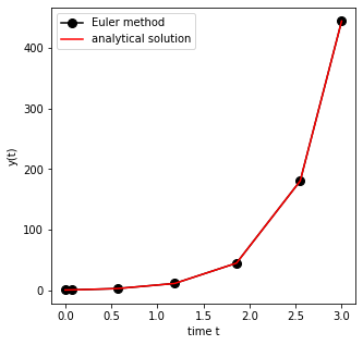
We first consider a simple linear ODE of the form
where \(c\) and \(k\) are parameters. The steady state \(x^0\) of the system can be straightforwardly calculated
To solve the system numerically, we must implement the function \(f(x,t) = c - k \cdot x\) into a user-defined {:raw-latex:`tt `python} function.
def exponential_growth(t, y):
    """
    The function implements the simple linear
    ODE dydt = k*y
    """
    return 2.0 * y
To integrate the system numerically, we need to specify the initial condition \(x^0 = x(t=0)\) and a timespan.
from scipy.integrate import solve_ivp
import numpy as np

# solve the ODE
y0 = 1.1
sol = solve_ivp(fun=exponential_growth, y0=np.array([y0]), t_span=[0, 3])

# plot both solutions
fig, ax = plt.subplots(nrows=1, ncols=1, figsize=(5,5))

ax.plot(sol.t, sol.y[0], 'ko-', markersize=8, label='Euler method')
ax.plot(sol.t, y0*np.exp(2.0*sol.t),'r-',label='analytical solution')
ax.set_xlabel('time t')
ax.set_ylabel('y(t)')
ax.legend(loc='upper left')
plt.show()
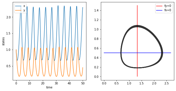
The Lotka-Volterra System
We want to implement the two-dimensional Lotka-Volterra System. A suitable function is
def lotka_volterra(t, x):
    """
    Implements the Lotka-Volterra System x is a two-dimensional vector
    """

    # define parameters
    X = x[0]
    Y = x[1]

    a = 1
    b = 2
    g = 1.5
    d = 2

    dxdt = a*X - b*X*Y
    dydt = g*X*Y - d*Y

    # the function returns the vector [fx, fy]
    return [dxdt, dydt]
First we have a look at state variables over time, i.e. we are looking at the oscillations of x and y through time.
The isoclines can be plotted as follows
import pandas as pd

# parameters for lotka volterra
a = 1
b = 2
g = 1.5
d = 2

# solve the ODE
y0 = [1, 1]
sol = solve_ivp(lotka_volterra, y0=y0, t_span=[0, 50], t_eval=np.linspace(0,50, num=1001))
# store solution in dataframe
s = pd.DataFrame(np.transpose(sol.y), columns=['x', 'y'])
s['time'] = sol.t

# plot solution
fig, (ax1, ax2) = plt.subplots(nrows=1, ncols=2, figsize=(10,5))

# plot timecourse
ax1.plot(s.time, s.x, label='x')
ax1.plot(s.time, s.y, label='y')

ax1.set_xlabel('time')
ax1.set_ylabel('states')
ax1.legend(loc='upper left')

# plot state space with nullklines

ax2.plot([d/g, d/g],[0, 3*a/b],'r-', label="fy=0")
ax2.plot([0, 2*d/g],[a/b, a/b],'b-', label="fx=0")
ax2.plot(s.x, s.y, 'k', alpha=0.8)
ax2.legend()
plt.show()
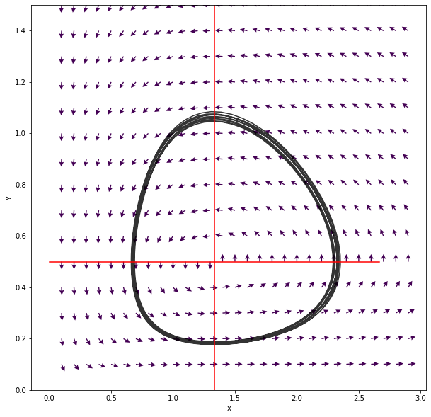
We can also have a more detailed look on the phase plane. A suitable
method are quiver plots (help(plt.quiver).
# solve the ODE
y0 = [1.0, 1.0]
sol = solve_ivp(lotka_volterra, y0=y0, t_span=[0, 50], t_eval=np.linspace(0,50, num=1001))
# store solution in dataframe
s = pd.DataFrame(np.transpose(sol.y), columns=['x', 'y'])
s['time'] = sol.t

x = np.arange(0.1,3,0.1); y = np.arange(0.1,3,0.1)
[xg,yg] = np.meshgrid(x,y)
n = np.size(x); m = np.size(x)
u = np.zeros([n,m])
v = np.zeros([n,m])

for i in range(n):
    for j in range(m):
        df = lotka_volterra(1, [xg[i,j],yg[i,j]])
        df = df/np.linalg.norm(df)
        u[i,j] = df[0]
        v[i,j] = df[1]

fig, ax = plt.subplots(nrows=1, ncols=1, figsize=(10,10))

h = ax.quiver(xg,yg,u,v,0.5, headwidth=5)
ax.plot(s.x, s.y, 'k-', alpha=0.8)
ax.plot([d/g, d/g],[0, 3*a/b],'r-')
ax.plot([0, 2*d/g],[a/b, a/b],'r-')
ax.set_ylim(0, 1.5)
ax.set_xlabel("x")
ax.set_ylabel("y")

plt.show()