04 Finite difference equations
(Lineare und nicht-lineare Abbildungen)
- discrete time
- rules for update of states
- also called: maps
\(x_{t+1} = f(x_{t})\)
Linear map (1D)
(Abbildung) First we look at the simplest case of maps, the linear map in 1 dimension
\(x_{t+1} = f(x_{t}) = R \cdot x_{t}\)
From a given initial state we can simulate the time evolution:
\(x_{0}\) (initial condition)
\(x_{1} = R \cdot x_{0}\)
\(x_{2} = R \cdot x_{1} = R^2 \cdot x_{0}\)
\(x_{3} = R \cdot x_{2} = \cdots = R^3 \cdot x_{0}\)
\(\cdots\)
We get a time series of states (trajectory in 1 dimensional state space).
steady state
An important question for dynamical systems are the steady states. Steady states of a map are defined via:
\(\bar{x}_{t+1} = \bar{x}_{t}\)
In case of the linear map this results in
\(R \cdot \bar{x} = \bar{x}\)
\(\bar{x} = 0\)
system behavior
Depending on the value of \(R\) different system behavior is observed in the linear map
- \(R > 1\) : growth
- \(R = 1\) : steady state (for all x)
- \(0 < R < 1\) : decay
- \(-1 < R < 0\) : alternating decay
- \(R = -1\): periodic cycle
- \(R < -1\): alternating growth
We can see the different possible modes in the following figure.
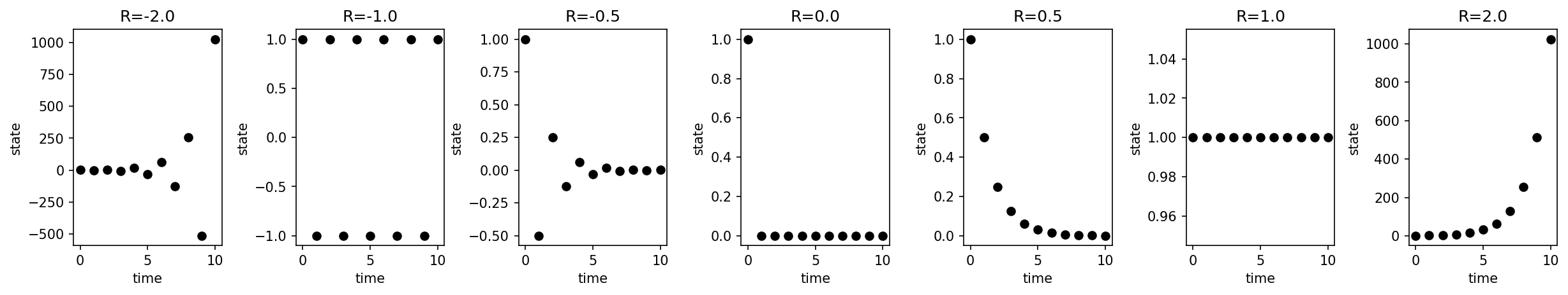
Simple linear map \(x_{t+1} = R \cdot x_{t}\)
graphical solution (web method)
An important tool for the analysis of 1 dimensional maps is the graphical analysis.
One plots the map function (\((x_{t}, f(x_{t})) = (x_{t}, x_{t+1})\) combined with the identity line.
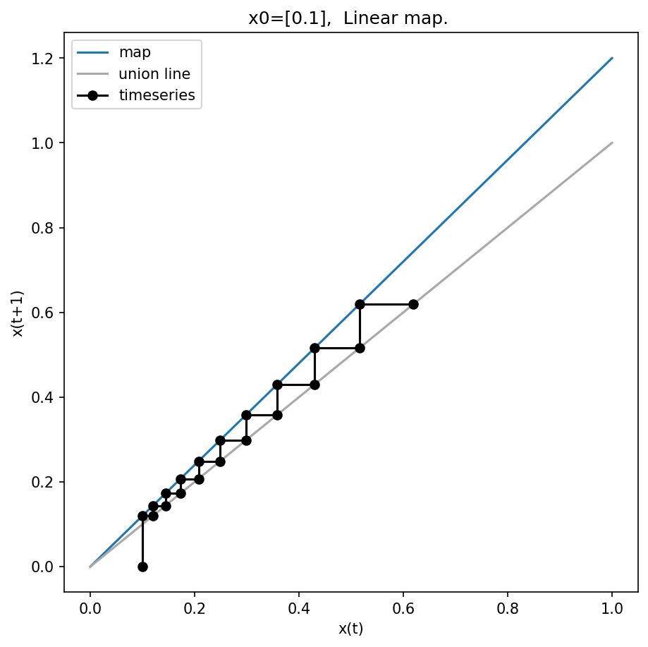
Graphical solution of linear map.
Nonlinear maps
(Nichtlineare Abbildung)
The linear map
\(x_{t+1} = R \cdot x_{t}\)
is for \(R > 1\) a simple model of exponential growth. But in reality resources are limited.
logistic map
A better description of growth processes with limitations is the logistic map, which
has an additional term restricting growth.
\(x_{t+1} = R \cdot x_{t} \cdot (1-x_{t})\)
\(0 \leq R \leq 4\)
The map is a function
\([0, 1] \rightarrow [0,1]\)
Example simulation
We will run an example starting from \(x_{0}=0.5\) (initial condition) with \(R=1.5\).
\(x_{0} = 0.5\)
\(x_{1} = \frac{3}{2} \cdot \frac{1}{2} \cdot(1 - \frac{1}{2})=\frac{3}{8}\)
\(x_{2} = \frac{3}{2} \cdot \frac{3}{8} \cdot(1-\frac{3}{8})=0.352\)
\(x_{3} = \cdots = 0.342\)
\(x_{4} = \cdots = 0.3375\)
\(\cdots\)
steady state
We calculate the steady state via
\(\bar{x}_{t+1} = \bar{x}_{t}\)
\(R \cdot \bar{x} \cdot(1-\bar{x}) = \bar{x}\)
\(R - R \cdot \bar{x} = 1\)
Resulting in
\(\bar{x}_{1} = 1-\frac{1}{R}\)
\(\bar{x}_{2} = 0\)
For our example (R=1.5) we get the steady state
\(\bar{x}_{2} = 1-\frac{2}{3} = \frac{1}{3}\)
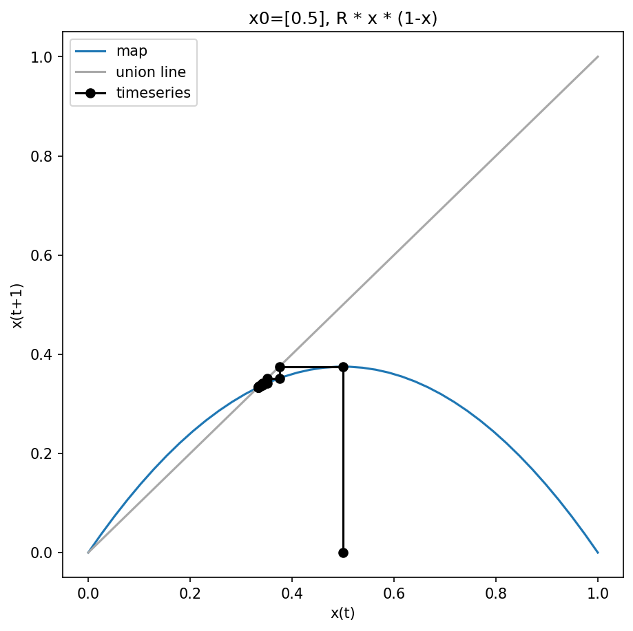
Graphical solution of logistic map
The steady states can be seen graphically in the web plot
- logistic map is a parabel
- crossings of map function \(f\) with union line
- corresponds to \(x_{t+1} = f(x_{t}) = x_{t}\)
Steady state analysis
We have found that the fix points / steady states in the system are
\(\bar{x}_{1} = 1-\frac{1}{R}\)
\(\bar{x}_{2} = 0\)
An important question is about stability of this fix points? The stability can be calculated by evaluating the derivative in the fix point