09 Sensitivity analysis
Review kinetic models of metabolism
- System of reactions with rate laws \(v_k(\vec{x}, \vec{p}) = f(\vec{x}, \vec{p})\) (\(k \in {1, ..., N_r}\)) which depend on metabolites \(x_i\) (\(i \in {1, ..., N_m}\)) and parameters \(p_m\) (\(i \in {1, ..., N_p})\)
- Stochiometric matrix \(N \in I\!R(N_m, N_r)\)
- Time evolution of \(\vec{x}(t)\) via system of ordinary differential equations from initial state \(\vec{x}_0\) via
- Steady state via
- Stability can be analysed using Jacobian matrix \(J = N \frac{d\vec{v}}{d\vec{x}}\)
Sensitivity
A sensitivity quantifies how changes in a parameter or state variable affect results.
A key concept is hereby the sensitivity of a function \(y = f(x)\) with respect to a parameter \(x\) defined as derivative
This sensitivity depends on the absolute value of the parameter: absolute sensitivity
Logarithmic sensitivity
Often the relative sensitivity or logarithmic sensitivity, which scales the sensitivity according to a given reference parameter \(x^0\).
An advantage is that logarithmic sensitivities are unit-less. But can be undefined for certain parameter/value combinations.
Example
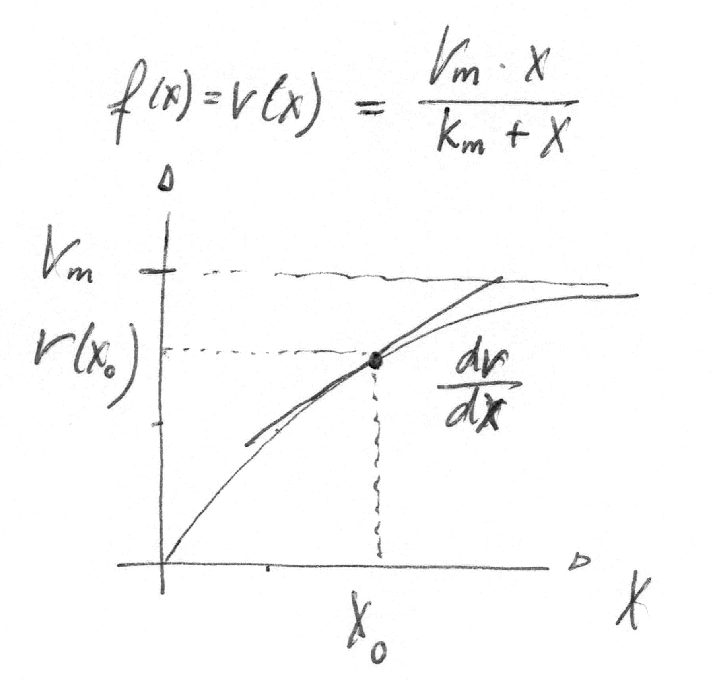
For instance we can calculate the sensitivity of a Michaelis-Menten rate equation \(v(x)\) on the metabolite concentrations x at a concentration \(x^0\)
The logarithmic sensitivities have an intuitive interpretation as the kinetic order of a reaction. For a Michaelis-Menten function, the logarithmic sensititivity with respect to the substrates ranges from
linear regime
\(x^0 \ll K_m \Rightarrow \frac{\partial \ln v}{\partial \ln x} \to 1\) (substrate concentration small compared to \(K_m\))
Compare to \(\frac{V_m \cdot x}{K_m + x} \to_{x << K_m} \frac{V_m}{K_m} \cdot x\)
saturation
\(x^0 \gg K_m \Rightarrow \frac{\partial \ln v}{\partial \ln x} \to 0\) (saturation, substrate concentration large compared to \(K_m\))
Metabolic Control Analysis (MCA)
- In metabolic networks the steady state variables, that is the fluxes and metabolite concentrations, depend on the value of parameters such as enzyme concentrations, kinetic constants (like Michelis-Menten constants).
- The effect of perturbations depends the place of the perturbation.
- MCA considers how a perturbation propagates through a metabolic network. Typically: how a change in enzyme concentration (or other parameter) affects the steady state with respect to metabolite concentrations and flux values.
- framework for studying the relationship between steady-state properties of a network of biochemical reactions and the properties of the individual reactions
- tool for analysis of control and regulation
- originally developed for metabolic networks, MCA has found application in signaling pathways, gene expression models, and hierarchical models
- metabolic networks are complex systems
MCA is conceptionally similar to classic sensitivity or control theory (from engineering).
The relations between steady state variables and kinetic parameters are usually nonlinear. MCA analyses small parameter changes around steady state.
Two distinct type of coefficients:
- elasticity coefficients are local coefficients pertaining to individual reactions. They can be calculated in any given state.
- control coefficients and response coefficients are global quantities. They refer to a given steady state of the entire system.
Elasticities
An elasticity coefficient quantifies the sensitivity of a reaction rate to the change of a concentration or a parameter while all other arguments of the kinetic law are kept fixed.
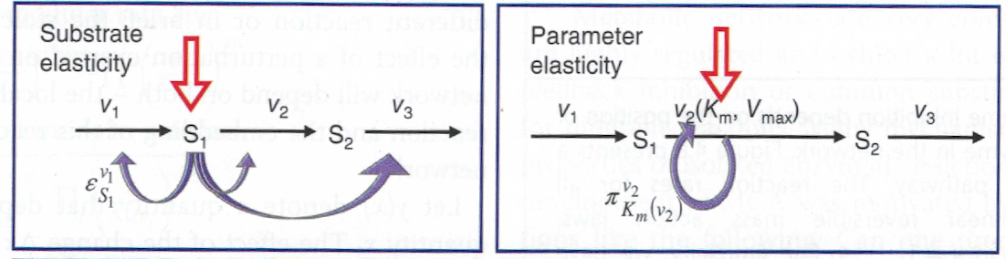
In MCA, the partial derivative of a reaction rate with respect to its substrate is called \(\epsilon\)-elasticity
More general, the sensitivity of the rate \(v_k\) of a reaction to the change of the concentration \(x_i\) of a metabolite is calculated by
The corresponding scaled elasticities are
A set of reactions and a set of metabolites results in an elasticity matrix \(\epsilon\). Note that the Jacobian matrix is \(J = N \cdot \epsilon\).
Examples
What are the logarithmic (normalized/scaled) sensitivities of the following functions with respect to the variable \(x\)
The \(\pi\)-elasticity is defined with respect to parameters \(p_m\) like kinetic constants, concentrations of enzymes, or concentrations of external metabolites
Control coefficients
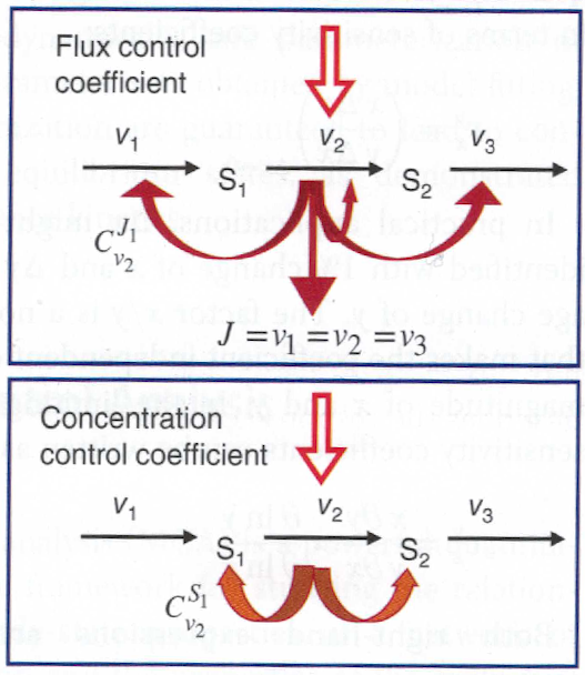
A control coefficient measures the relative steady state change in a system variable, e.g. pathway flux \(J_k\) or metabolite concentration \(x_i\). The two main control coefficients are the flux and concentration control coefficients.
Control coefficients are defined in a stable steady state of the metabolic system, characterized by steady state \(x^{ss}\) concentrations and fluxes \(\vec{J}\).
Any sufficiently small perturbation of an individual reaction rate \(v_k \to v_k + \Delta v_k\) drives the system to a new steady state in close proximity with \(\vec{J} \to \vec{J} + \Delta \vec{J}\) and \(\vec{x^{ss}} \to \vec{x^{ss}} + \Delta \vec{x^{ss}}\).
A measure of the change of fluxes and concentrations are the control coefficients.
Flux control coefficients
The flux control coefficient for the control of rate \(v_k\) over flux \(J_j\) is defined as
The flux control coefficient quantifies the control that a certain reaction \(v_k\) exerts on the steady state flux \(J_j\).
The rate change \(\Delta v_k\) is caused by the change of a parameter \(p_k\), that has direct effect solely on \(v_k\)
Such a parameter might be the enzyme concentration, a kinetic constant, or the concentration of a specific inhibitor or activator.
Concentration control coefficient
The concentration control coefficients specify how the steady state concentrations change due to a perturbation of a parameter (typically an enzyme concentration) that effects one or more fluxes.
Response coefficients
- The steady state is determined by the values of the parameters.
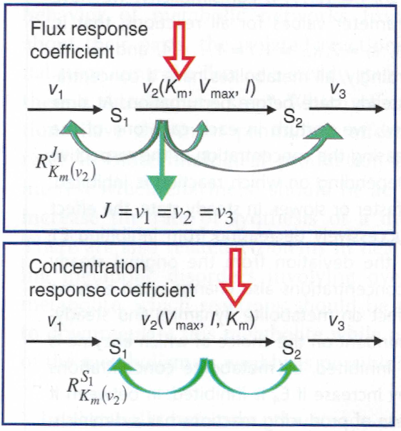
- The response coefficients express the direct dependency of steady state variables on parameters.
Flux response coefficient
Response of steady state flux to parameter perturbations
Concentration response coefficient
Response of steady state concentration to parameter perturbation
Theorems of MCA
Summation Theorems
The summation theorems make a statement about the total control over a certain steady-state flux or concentration.
The flux control coefficients fulfill
That means that all enzymatic reactions can share the control over this flux.
The concentration control coefficients fulfill
The control coefficients of a metabolic network for one steady-state concentration are balanced. Enzyme can share control, but some exert negative control while others exert positive control.
Connectivity Theorems
Flux control coefficients and elasticities are related by
The sum runs over all rates \(v_k\) for any flux \(J_j\)
The connectivity theorem between concentration control coefficients and elasticities is
Again, the sum runs over all rates \(v_k\), while \(x_h\) and \(x_i\) are the concentrations of two fixed metabolites.
References & further reading
- https://en.wikipedia.org/wiki/Metabolic_control_analysis
- Klipp et al, Systems Biology - A textbook, chapter 4.2 - Metabolic control analysis
- Reder, C. “Metabolic control theory: a structural approach.” Journal of theoretical biology vol. 135,2 (1988): 175-201. doi:10.1016/s0022-5193(88)80073-0
- Kacser, H, and J A Burns. “The control of flux.” Symposia of the Society for Experimental Biology vol. 27 (1973): 65-104.
- Heinrich, R, and T A Rapoport. “A linear steady-state treatment of enzymatic chains. General properties, control and effector strength.” European journal of biochemistry vol. 42,1 (1974): 89-95. doi:10.1111/j.1432-1033.1974.tb03318.x