11 Signaling
Previously metabolism
describing mass flow and metabolic flux
Signaling
In signal transduction we focus on information transfer from input signal (internal or external) to output, i.e. cellular response.
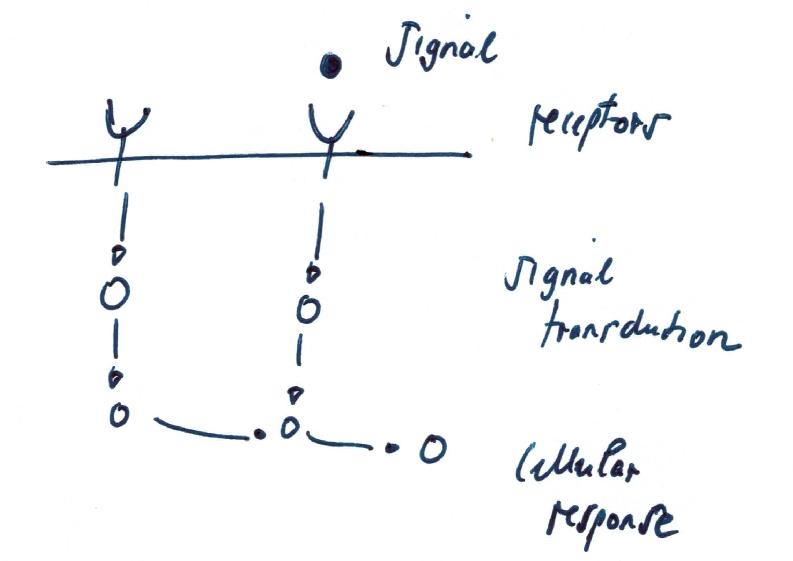
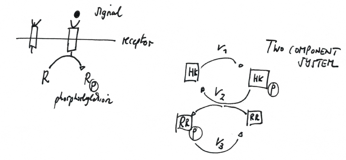
General principle of activation of response regulator \(R\) by signal \(S\): signal binds to receptors activating a signal transduction cascade/path which ultimately results in a cellular response.
Main biological steps
- receptor binding
- complex formation
- protein modification (phosphorylation & dephosphorylation)
- activation of gene transcription
Typical signals are: growth hormones, pheromones, heat, osmotic pressure, oxidative stress or substances.
Phosphorylation cycle
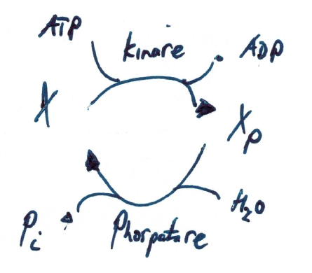
One of the most important signaling motives are protein phosphorylation cycles, i.e., a post-translational modification of a protein in which an amino acid residue is phosphorylated by a protein kinase, and dephosphorylated by a protein phosphatase.
Phosphorylation is a very common mechanism for regulating the activity of enzymes and is the most common post-translational modification. Other modifications are for instance glycosylation, acetylation or lipidation and can be modelled in a very similar manner.
Phosphorylation changes the structural conformation of the protein, the phosphorylated protein has a modified function (e.g. phosphorylation may activate or deactivate a protein)
Important examples are two-component signaling systems and mitogen-activated protein kinase (MAPK or MAP kinase) systems (as well as many others, e.g., phosphorylation of enzymes).
Simple models follow mass-action kinetics. For example the following simple phosphorylation cycle where the kinase activity represents the signal \(S\), and the activity of the phosphatase is assumed to be constant (and included in the rate constant \(k_2\).)
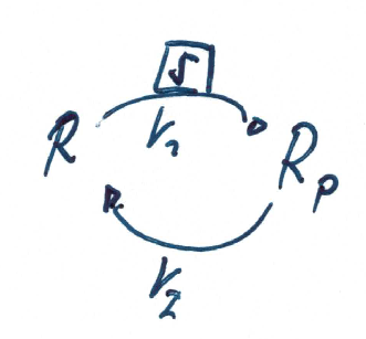
The system exhibits mass conservation \(R_p + R = R^T\), where \(R^T\) denotes the amount of total protein.
Steady state
Steady state of the system is given by
which is a Michaelis-Menten like response
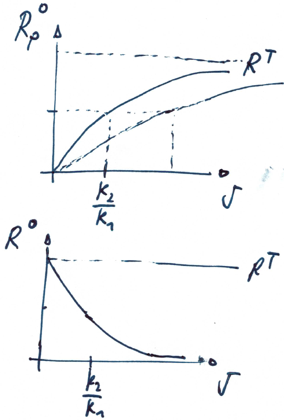
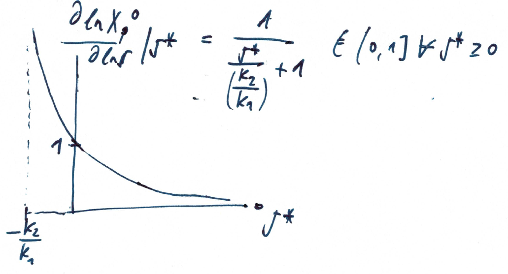
Note that the dependence on the kinase activity (signal) is hyperbolic, whereas the dependence on total protein is linear.
Sensitivity of steady state
Dependency on signal
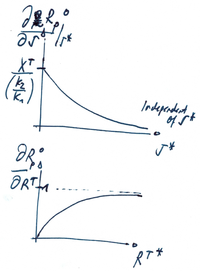
Dependency on total response regulator
Two-component system
A two-component regulatory system serves as a basic stimulus-response coupling mechanism to allow organisms to sense and respond to changes in many different environmental conditions.
Two-component signaling systems typically consist of
- (membrane-bound) histidine kinase (HK) that senses a specific environmental stimulus (typically homodimeric transmembrane proteins containing a histidine phosphotransfer domain and an ATP binding domain)
- corresponding response regulator that mediates the cellular response, mostly through differential expression of target genes (may consist only of receiver domain, but mostly receiver and output domain, often involved in DNA binding)
- two-component systems serve as a basic stimulus-response coupling mechanism to allow organism to sense and response to changes in many different environmental conditions.
- overall level of phosphorylated response regulator ultimately controls its activity
- many HKs are bifunctional and possess phosphatase activity against response regulator
- most common in bacteria
Important examples
- bacterial chemotaxis
- E.coli osmoregulation (EnvZ/OmpR)
- B.subtilis sporulation
Robustness of two-component systems
The cellular environment fluctuates and protein expression is stochastic. Cells evolved mechanisms to cope with such fluctuations. A well known example is the robustness of (some) two-component systems with respect to fluctuations in the total amounts of proteins.
To model a two-component system (using mass-action kinetics), we consider the dynamics of the histidine kinase \(H\) and the response regulator \(R\). Both exist in phosphorylated and unphosphorylated form. The ODEs are
- mass action kinetics
- \(H\): histidine kinase
- \(R\): response regulator
mass conservation: \(H + H_p = H^T\) and \(R + R_p = R^T\)
steady state solution can be calculated, but lengthy quadratic equation.
In many 2 component systems, the (unphosphorylated) sensor kinase also acts as a phosphatase for the response regulator. This results in redundancy in the system: the phosphorylated form activates the response regulator, the unphosphorylated form deactivates the response regulator.
A possible reason was to prevent residual (auto- or unspecific) activation of the response regulator. The equations, however, show that the effect is more profound.
At steady state we know that \(v1 = v3\). Hence, if the dephosphorylation reaction is
the steady state solution for the response regulator is
The resulting expression is independent of the expression of the proteins \(R\) and \(H\). This is often termed perfect adaption or integral feedback.
Ultra-sensitivity
An ultrasensitive response describes a response that is more sensitive to changes in input than the hyperbolic Michaelis-Menten response.
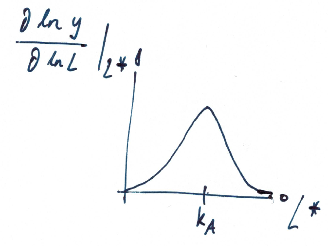
Ultrasensitivity was first (heuristically) described by A. Hill in 1910 to describe the sigmoidal O2 binding curve of haemoglobin. The hill equation is
\(y\) denotes some output (such as the fractional binding), \(L\) the concentration of a ligand, \(k_p\) a proportionality constant, \(K_A\) the half-saturation constant, and \(n\) the Hill coefficient.
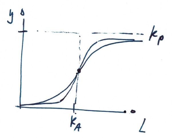
Increasing n results in steeper sigmoidal response.
What is the logarithmic sensitivity of the output with respect to the ligand concentration?
A mechanistic model for ultrasensitivity was proposed by Goldbeter and Koshland, the Goldbeter-Koshland switch. The switch arises if the reactions in a protein phosphorylation cycle are close to saturation. Similar to equation
The solution provides the Goldbeter-Koshland function, a sigmoidal response curve in steady state.
To calculate the steady-state solution \(R_p^0 = f(S)\) is straight-forward but lengthy. It is much simpler to calculate the inverse function \(S = g(R_p^0)\) and plot this function.
There are now several other known mechanisms that result in ultrasensitivity (see articles by Ferrel and Ha).
References & further reading
- https://en.wikipedia.org/wiki/Post-translational_modification
- https://en.wikipedia.org/wiki/Two-component_regulatory_system
- https://en.wikipedia.org/wiki/Goldbeter%E2%80%93Koshland_kinetics
- Stock, Ann M., Victoria L. Robinson, and Paul N. Goudreau. “Two-component signal transduction.” Annual review of biochemistry 69.1 (2000): 183-215.
- Klipp et al, Systems Biology - A textbook, chapter 12.2 - Signaling pathways
- Batchelor, Eric, and Mark Goulian. “Robustness and the cycle of phosphorylation and dephosphorylation in a two-component regulatory system.” Proceedings of the National Academy of Sciences 100.2 (2003): 691-696.
- Ferrell Jr, James E., and Sang Hoon Ha. “Ultrasensitivity part I: Michaelian responses and zero-order ultrasensitivity.” Trends in biochemical sciences 39.10 (2014): 496-503.
- Ferrell, James E., and Sang Hoon Ha. “Ultrasensitivity part II: multisite phosphorylation, stoichiometric inhibitors, and positive feedback.” Trends in biochemical sciences 39.11 (2014): 556-569.
- Ferrell Jr, James E., and Sang Hoon Ha. “Ultrasensitivity part III: cascades, bistable switches, and oscillators.” Trends in biochemical sciences 39.12 (2014): 612-618.